Enterprise AI APIs for Semiconductor & Edge Computing

Cosmic
Dorito

We build hosted B2B cloud APIs for automated semiconductor wafer inspection, powered by physics-informed neural networks.

Our platform turns raw sensor data into actionable intelligence. From distributed edge scheduling to LLM document pipelines, every claim below traces to a measurable, production-ready system.

942 Mbit/s
Measured cluster fabric, iperf3, zero retransmits
20.96 GFLOPS
HPL/Linpack across two Pi 4 nodes — 2.05× scaling
~74 µs
Scheduler decision cost per task, measured
99.82%
Bearing fault accuracy, four classes under variable load
0.193 W
FPGA design on-chip power, post-synthesis, deployed
National Institute of Ocean Technology TVS Motor Company Hyundai Motor India Amrita Vishwa Vidyapeetham
Research & Development partnerships and study — institutional experience, not endorsement.
01

Our Products

01 Ongoing · Core Platform

Adaptive task partitioning on a Raspberry Pi edge cluster

A coordinator/worker runtime that schedules CNN inference across SBC nodes using an online cost model — live capability, queue backlog, communication cost, and thermal derating — on a measured Gigabit fabric with K3s and Prometheus/Grafana underneath.

105/105 split · LBE 1.000 ~74 µs/task MobileNet-v2K3s
Case study →
AdaptiveMCT pi4-main1pi4-main2 Pi 3 · next GigE 10.0.0.x
02 Hosted API

When do physics-informed neural networks actually help?

Sparse on-chip thermal field reconstruction under power-model and nonlinear-leakage uncertainty. Three controlled studies against classical data assimilation, a physics-embedded Green’s-basis PINN that fixes spectral-bias collapse, and a closed-form D-optimal sensor placement.

0.60 K · D-optimal, EV6 2.3× vs next-best SC-GB-PINNcode + seeds released
Case study →
8 sensors → full field + leakage coefficient
03 R&D · NIOT

Mini ROV with multi-sensor telemetry & fault-tolerant optical link

Built at the National Institute of Ocean Technology, Deep Sea Technology Group: a Raspberry Pi 5 vehicle with T200 thrusters, depth and motion sensing, RS485 telemetry, and an operator UI — plus a visible-light link that survives corrupted bits by redundancy and retransmission.
recovers from injected errors RS485Pi 5T200 + ESC
Case study →
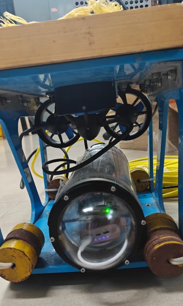
Mini ROV prototype: thrusters above a transparent pressure housing
04 Enterprise Case Study · TVSM R&D

LLM patent-intelligence pipeline for TVS Motor

Two-layer document intelligence: deterministic parsing for metadata, grounded LLM reasoning for engineering fields — with full-document OCR arbitration, design-patent handling, guard-railed claim cleanup, per-field confidence, and team routing. Deployed internally for TVSM R&D teams.

deployed internally Azure OpenAITesseract OCRStreamlit
Case study →
PDF+OCR regex layer LLM layer report
05 Signal Processing · Deep Learning

Bearing fault diagnosis with frequency-domain attention

FD-MRA: multi-resolution attention over vibration spectra with trainable frequency masks and rotary position embeddings, fused with a 1-D time-domain CNN through a 256-D bottleneck — classifying four fault classes across 0–3 HP variable load at a latency that runs on the machine rather than in the cloud.

99.82% accuracymacro-F1 0.9982 0.8 ms inferenceRoPE attention
Case study →
learned masks attend fault bands across loads
06 Completed · PCB validated

Fully analog electronic stethoscope

No microcontroller anywhere: an electret chestpiece into op-amp gain stages, a 50 Hz notch, and three 4th-order Sallen–Key bandpass paths that isolate heart, lung, and murmur bands — designed on paper, simulated, built, and verified against a bench frequency-response analyzer.
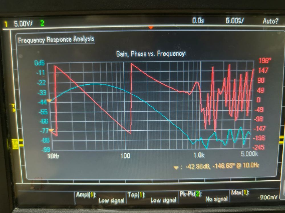
notch measured at 49.8 Hz 3 bandsSallen–Key ×3PCB
Case study →
Oscilloscope frequency-response analysis of the stethoscope filter chain
+ Completed · On hardware

FPGA memory game on Basys-3

Modular Verilog — FSM game logic, LFSR sequences, debounced 4×4 keypad, clock division from 100 MHz, seven-segment driver. Verified in ModelSim, taken through Vivado synthesis, implementation and DRC sign-off, then deployed to the physical XC7A35T board.

0.193 W on-chip0.56% FF util.
02

R&D Experience

Apr 2026

Research Intern — Deep Sea Technology Group

National Institute of Ocean Technology (NIOT), Ministry of Earth Sciences, Chennai
  • Developed a mini remotely operated vehicle: Raspberry Pi 5 control, Blue Robotics T200 thrusters with ESCs, depth/pressure sensing, Xsens motion sensing, RS485 telemetry to a laptop operator UI, packaged in a 4-inch pressure housing.
  • Built a fault-tolerant optical wireless link on Arduino: triple-redundancy encoding, majority-vote decoding with correction masks, timeouts and automatic retransmission.
Case study →
May – Jun 2026

AI/ML Intern

TVS Motor Company, Hosur
  • Built and shipped an LLM-based patent-intelligence pipeline — deterministic metadata extraction plus grounded LLM analysis, OCR for scanned and design patents, confidence scoring and team routing.
  • Deployed internally for TVSM R&D teams with a Streamlit batch UI and a one-command installer.
Case study →
May – Jun 2025

Engineering Intern

Hyundai Motor India Limited
  • Evaluated automated assembly workflows for HS220 and HS160L six-axis robotic arms — cycle-time distributions, motion-sequencing logic, throughput constraints.
  • Mapped kinematic envelopes, workspace limits and collision-avoidance zones.
2023 – 2027

B.Tech, Electronics & Communication Engineering — AI/ML minor

Amrita Vishwa Vidyapeetham, Coimbatore
  • Core CGPA 8.33 · minor CGPA 9.26.
  • NPTEL Embedded Systems Design (IIT Kharagpur) — Elite, top 1%.
03

Research

Manuscript · Aug 2026

When Do Physics-Informed Neural Networks Help? Sparse On-Chip Thermal Field Reconstruction under Power-Model and Nonlinear-Leakage Uncertainty

S. Sanjay Subramanyan, S. Sahithya, M. Suprithi, J. P. Anitha. Three controlled studies separating power-model from physics-model uncertainty; a self-consistent Green’s-basis PINN; a training-free D-optimal sensor placement; and a decision rule for practitioners. All code, seeds and metrics released.

04

About Cosmic Dorito

Cosmic Dorito is an early-stage AI startup building hosted B2B cloud APIs for automated semiconductor wafer inspection and physics-informed machine learning. Our work sits where models meet hardware: a model that has to run on a specific device, a sensor whose physics shapes the estimator, a scheduler whose cost model has to survive real network latency.

The pattern across our platform is the same — build the system end to end, instrument it, and let the measurements decide. Sometimes that means reporting that a classical Gaussian process ties the neural network at a fraction of the compute, and saying so. We would rather ship the honest number than the flattering one.

05

Platform Capabilities

AI / ML
PyTorch · TensorFlow · MATLAB · CNNs · SNNs · PINNs · Gaussian processes · attention architectures
Edge / Systems
Distributed scheduling · Raspberry Pi clusters · K3s · Prometheus/Grafana · HPL benchmarking · TCP protocol design
LLM Engineering
Azure OpenAI · grounded extraction · OCR pipelines (Tesseract) · validation & guardrails · Streamlit apps
Embedded
C/C++ · Assembly · Arduino · Raspberry Pi · RS485 · sensor integration · Keil µVision
RTL / FPGA
Verilog · Vivado synthesis→DRC sign-off · ModelSim · Basys-3 deployment
Electronics
Active filter design · op-amp circuits · LTSpice · ANSYS HFSS · SEMulator3D · PCB design (EasyEDA) & fabrication · bench validation
06

Get in touch

Open to enterprise API access, partnership inquiries, and pilot programs for our semiconductor inspection platform.
← All products

Adaptive task partitioning across distributed SBC nodes

Core platform — a runtime that turns a validated Raspberry Pi cluster into an online scheduler for edge-AI workloads.

Status: ongoing Report: 9 Aug 2026
01 — Overview

Make cheap boards behave like one machine that knows itself

Two phases. First, recreate a reference Raspberry Pi cluster stack — Ethernet fabric, HPL/Linpack, K3s, Prometheus/Grafana — and measure everything, so the platform itself is validated rather than assumed. Second, build a coordinator/worker runtime on top of it that assigns each inference task to the node expected to finish it first.

942 Mbit/s fabric (Wi-Fi: 26) 0.31 ms avg RTT 10.20 → 20.96 GFLOPS, 2.05× 10⁵ / 105 task split, LBE 1.000 ~74 µs scheduler overhead/task
02 — Problem

Why scheduling on cheap edge hardware is its own problem

Cheap heterogeneous single-board computers on commodity Ethernet break the assumptions cluster schedulers usually make. Node capability differs and drifts; fanless boards thermally throttle under sustained load; and moving data is expensive enough that the network term belongs inside the placement decision, not in a footnote. The scheduler has to learn what nodes can actually do — online, from the tasks themselves — and it has to decide in microseconds, because on a fast fabric a slow scheduler is the bottleneck.

The workload model is task-level partitioning: each webcam frame runs full MobileNet-v2 inference on one node. Splitting a single inference across nodes would shuttle intermediate feature maps over commodity Ethernet — the measured network baseline says that trade is a loss, so the design keeps every task whole and lets placement do the work.

03 — Validated substrate

Measure the platform before trusting it

The cluster is dual-homed by design: the laptop stays on Wi-Fi for management, while all worker traffic rides a dedicated Gigabit Ethernet data plane (10.0.0.x). The reference recreation follows Jeff Geerling’s public Pi-cluster automation and benchmark workflow, then verifies each layer manually.

LayerMeasuredMeaning
Ethernet fabric942 Mbit/s · 0.31 ms · 0 retr.iperf3 + ping — the scheduler’s communication term is grounded in this
Wi-Fi (same hardware)≈26 Mbit/s36× slower — why the data plane is wired
HPL / Linpack, 1 × Pi 410.20 GFLOPSReference figure for the board class is ≈11.9 — right order, validated
HPL / Linpack, 2 × Pi 420.96 GFLOPS · 2.05×Near-linear scaling for a compute-bound kernel
K3s2 nodes Ready · 4 replicas 2+2Orchestration and self-healing verified
Prometheus + Grafanalive node dashboardsCPU, load, memory, disk, temperature during experiments
All values measured on this cluster and recorded in the project report (Aug 2026).

Legacy distributed benchmarks carried forward as baselines: prime counting speeds up 1.696× → 1.578× as workloads grow (coordination overhead is visible, then amortized), and a 4000×4000 matrix multiply runs 1.32× faster distributed — a more honest proxy for AI-style arithmetic than embarrassingly parallel primes.

04 — Scheduler design

AdaptiveMCT: minimum estimated completion time, learned online

Taskwork W · data D
Node statecapability C (EWMA) · queue · B, L · temp T
EstFinish(queue+compute)/Ceff + comm
Pick mintie-window spread
Executetelemetry → CSV

For each task the coordinator estimates every candidate node’s finish time — computation, current backlog, communication cost from measured bandwidth and latency, and a thermal derating factor that shrinks a node’s effective capability past a warning threshold and floors it near throttle. The most distinctive runtime feature is exactly that derating: fanless boards get protected before the silicon throttles them.

  • Wire protocol: length-prefixed JSON over TCP — every receive reads one whole message; the control path stays deterministic.
  • Workers are plug-and-play: start the process, get profiled on real workload, join mid-run. Failed tasks are requeued for self-healing.
  • Two baselines isolate the contribution: RoundRobin (ignores all state) and CapabilityWeightedStatic (initial estimate, never adapts).
  • Capability C is learned online and smoothed with EWMA — no hand-assigned node scores anywhere.
05 — Measured results

The current cluster behaves exactly as it should

MetricValueImplication
Task split, 210-task MobileNet-v2 run105 / 105No node favored when cost estimates tie
Load-balance efficiency1.000Tie-spreading logic works
Scheduler overhead~74 µs / taskLight enough for real-time use — decisions in microseconds, not milliseconds
Network + scheduling overhead~1.4 ms (~2%)Communication is not the bottleneck on this workload
Learned node capabilitieswithin 1.5%Identical hardware converges to a natural tie
06 — What this doesn't show yet

On identical nodes, the adaptive policy ties the baselines — by design

Read this before the numbers above

The current measured platform is two identical, cool Pi 4 nodes. On that hardware there is no heterogeneity to exploit, so AdaptiveMCT correctly ties RoundRobin and the static baseline — a validation of scheduler neutrality, not evidence of advantage. The expected win appears when Pi 3 nodes introduce genuine capability differences and when thermal stress activates the derating path. Those experiments are pending, and the report says so explicitly.

This is deliberate scientific sequencing: establish a correct, perfectly balanced baseline first, so any separation measured later is attributable to the policy rather than to platform noise.

07 — Roadmap

The experiments that separate the policies

  • Add Raspberry Pi 3 nodes — genuine heterogeneity, non-trivial policy separation.
  • Thermal workload — validate proactive derating on fanless boards where throttling is physically real.
  • Communication-heavy tasks — force the network term to earn its place in the cost model.
  • Ablations (thermal / communication / online-learning off) and multi-run statistics with variance.
  • Power measurement (USB meter or INA219) → energy-aware scheduling and GFLOPS/W.
← All products

When do physics-informed neural networks help?

Sparse on-chip thermal field reconstruction under power-model and nonlinear-leakage uncertainty. Manuscript, August 2026; all code, seeds and metrics released.

01 — The question

Not “are PINNs good” — when do they earn their compute?

A deployed chip exposes a handful of noisy on-die sensors, and the physics model driving any reconstruction is itself wrong: the power map is a nominal estimate, and leakage rises nonlinearly with temperature. The chip-thermal PINN literature demonstrates accurate forward analysis — but rarely compares against the classical alternative: solve the nominal physics, fit a Gaussian process to the sensor residual, add it back. This work stages that comparison honestly, three ways.

2.5-D steady-state model · 256×256 FDM truth 6-block 95 W chip + published 19-block Alpha 21264 (EV6) floorplan σ = 0.5 K sensor noise · 5 seeds everywhere
02 — Study 1 · linear regime

Under smooth power-model error, classical assimilation wins

Method (N = 20 sensors)ρ = 0%5%10%15%20%
PINN0.4240.4360.4830.5060.601
Physics-mean GP (assimilation)0.2140.3450.4750.6290.574
Physics only (no sensors)1.0862.4075.5528.55511.617
Field MAE [K] vs per-block power mismatch ρ, mean over five seeds. Best per column in accent.

The GP matches or beats the PINN at four of five mismatch levels — while running in under a second on a CPU against minutes on a GPU. Two to three orders of magnitude in compute for the same accuracy. In the smooth, linear regime the network confers no benefit, and the paper says so plainly.

03 — Study 2 · nonlinear leakage

Make the physics nonlinear and sensing scarce — the verdict flips

Temperature-dependent leakage is a positive feedback: heat raises leakage, which raises heat. Model it as an unknown coefficient β, drop to eight sensors, and the PINN — treating β as a trainable parameter constrained through the coupled residual — holds nearly flat (0.82–1.09 K) while pure physics degrades eighteen-fold and even the GP triples (0.40 → 1.34 K). The curves cross near β* ≈ 0.10.

PINN MAE 0.82–1.09 K across β* 0→0.12 β̂ recovered: 0.001→0.090 tracking truth monotonically PhysGP: 0.40→1.34 K · physics-only: 19.3 K

Uniquely, the PINN also returns a physical quantity no baseline can produce: the leakage coefficient itself, recovered from eight noisy sensors while reconstructing the field. Robustness held under an independent bilinear FEM reference (margin widens: 0.95 vs 1.33 K), doubled sensor noise (β̂ within ±0.003), and a five-member deep ensemble whose predictive σ brackets actual error.

04 — Study 3 · complex floorplans

A vanilla PINN collapses on the real floorplan — so embed the physics

On the published 19-block EV6 layout the freeform PINN fails outright — spectral-bias collapse to ≈8 K MAE even with the physics exactly known. The fix is architectural: precompute each block’s Green’s-function response once, write the field as a per-block Green’s expansion, and let leakage live on the same physical basis, solved to self-consistency inside the forward pass (SC-GB-PINN). Hard physics constraints, Nblocks+1 free parameters.

Method (β* = 0.12, FEM truth)SimpleSixEV6 (19 blocks)
Physics-mean GP1.322.57
Vanilla PINN1.418.04
GB-PINN (prior only)1.202.34
SC-GB-PINN1.011.01
Field MAE [K], five seeds. SC-GB-PINN: 2.3× better than next-best on EV6; β̂ = 0.12 / 0.10 (true 0.12).
Kept deliberately in the paper

At β* = 0 the SC-GB-PINN is not the best method (0.57–0.76 K vs 0.31–0.40 K for GP and GB-PINN) — its leakage machinery is dead weight when there is nothing to infer. The win is regime-specific, and reporting where a method loses is what makes the comparison believable.

05 — Where to put the sensors

The same basis answers a second question, for free

Because SC-GB-PINN reduces reconstruction to a few per-block parameters, its sensitivity at any location is available in closed form — so choosing the eight positions that maximize the Bayesian D-optimal criterion needs no training at all. On EV6 that drives error to 0.60 K — the lowest in the work — and 0.97 K on the simple chip, while shrinking variance roughly six-fold. And a cautionary measured result: clustering all sensors on the hotspots is catastrophic for the statistical baseline (19→24 K), because it starves the cool interior. Coverage, not intuition, matters — the criterion balances it automatically.

06 — Decision rule

What a practitioner should actually do

  • Smooth model error, adequate sensing → physics-mean Gaussian process. Equal accuracy at negligible cost, no training, trivial to deploy.
  • Strong nonlinearity, sparse sensing, or a parameter you need → PINN. Stays accurate where residual-smoothing fails and returns an interpretable coefficient as a by-product.
  • Complex multi-hotspot floorplans → embed the physics in the architecture (Green’s basis); a freeform network cannot fit the field at all.

The mechanism generalizes: a smoother treats physics as fixed and interpolates what sensors leave over; a PINN reshapes the physics through a trained parameter. Flexibility is dead weight exactly when classical methods already fit the physics.

07 — Limitations

Stated plainly, as in the paper

  • 2-D and simulation-based — a real published processor floorplan, cross-checked against an independent FEM solver, but not measured silicon or a 3-D package.
  • Assumes a known floorplan and nominal power map — a design-time estimator, not a black-box learner.
  • The leakage law is a controlled positive-feedback model; temperatures exceed realistic junction limits to make the nonlinearity visible.
  • No runtime speedup is claimed; reconstruction is treated as estimation.
← All products

Mini ROV & a light link that refuses to give up

Research internship, Deep Sea Technology Group, National Institute of Ocean Technology (Ministry of Earth Sciences), Chennai — April 2026.

Two projects, one monthPrototype · surface-testedDemo video ↗
01 — The vehicle

Propulsion, sensing, communication and control in one platform

The Mini ROV integrates Blue Robotics T200 thrusters with ESCs, a depth/pressure sensor, an Xsens motion sensor, and a Raspberry Pi 5 controller inside a 4-inch pressure housing — talking to a laptop operator station over RS485, chosen for robust long-distance wired communication.

Mini ROV: T200 thrusters mounted above the transparent 4-inch pressure housing, tether coiled behind
The prototype: thrusters, frame, and the sealed electronics housing. Photo from the internship report.
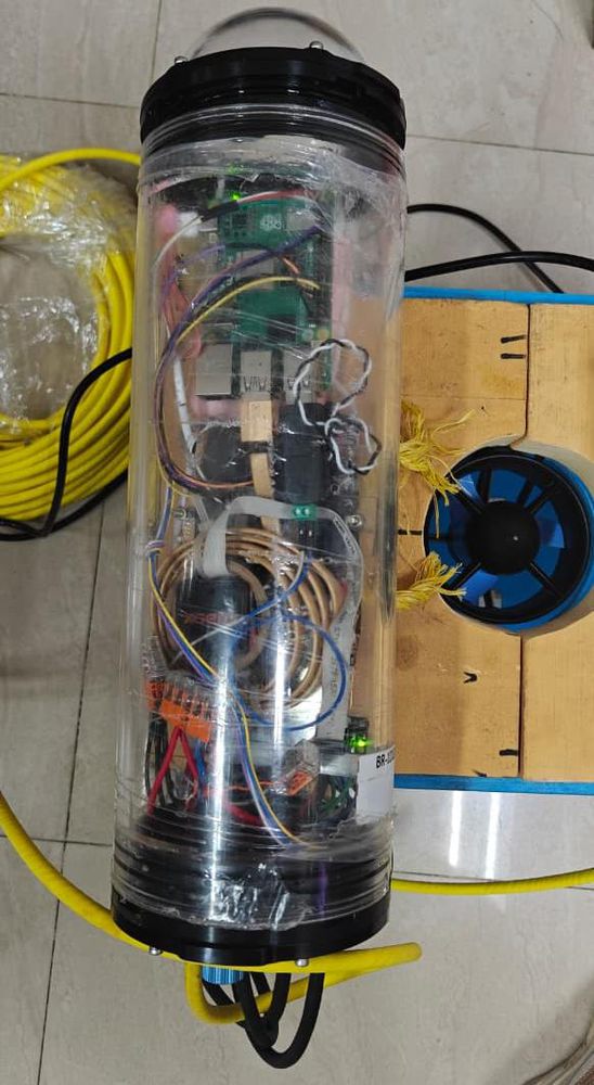
Inside the pressure housing: Raspberry Pi 5, wiring and power electronics
Inside the housing: Pi 5, buck-converted power (20 V bus for thrusters), sensor wiring.

My work was hardware integration, software interfacing and the operator UI: acquiring depth and motion data on the Pi, streaming telemetry to the laptop interface in real time, and carrying operator commands back down to the propulsion system.

02 — System architecture

Four subsystems, deliberately modular

Sensorsdepth/pressure · Xsens motion
Raspberry Pi 5acquisition · control
RS485 linkbidirectional telemetry
Operator UIlive readouts · commands

Each subsystem was integrated independently against the same interfaces — which is what made a one-month build feasible, and what the report credits for maintainability. Power design: a 20 V source for the thrusters through ESCs, with the Pi 5 fed by a buck converter so control stays stable while motors draw current.

03 — The optical link

Visible light as a wire — then make it survive corruption

The companion project: optical wireless communication on Arduino Uno — an LED transmitter and photodiode receiver on AltSoftSerial, run deliberately slow (300 bps on the optical channel) for stability. The interesting part is the fault tolerance added on top:

  • Triple-redundancy encoding — every byte transmitted three times.
  • Majority-vote decoding with a correction mask that records exactly which bits were repaired.
  • Timeouts and automatic retransmission — up to five attempts before giving up.
04 — Proof it works

Watch it fail twice and still deliver

From the loopback test log in the report — ambient interference corrupts the message on two attempts; bit-level correction plus retransmission recovers it exactly on the third:

Optical loopback with automatic retransmission on error
--- New message: "Rithish" ---
Attempt 1/5
  Char 0 corrected bits: 4 6 · Char 1: 3 5 6 · Char 2: 5 6 7
  Mismatch: sent="Rithish", received="Raÿÿÿ"
>>> Retransmitting in 200 ms...
Attempt 2/5
  Char 0: 1 6 · Char 2: 2 3 4 7 · Char 3: 6 7 · Char 4: 4
  Mismatch: sent="Rithish", received="0i00000"
>>> Retransmitting in 200 ms...
Attempt 3/5
  Char 4 corrected bits: 0 · Char 6 corrected bits: 3
>>> SUCCESS: Message received correctly.
Message successfully transmitted after 3 attempt(s). Final received: "Rithish"

The log makes the design case better than prose could: single-shot transmission fails in ambient light, and the redundancy + ARQ layer turns an unreliable channel into a reliable one.

05 — Limitations

What was and wasn't tested

  • Underwater facilities weren’t available during the internship — the ROV was validated by surface-level functional testing: all subsystems integrated, telemetry and commands verified end to end. Underwater performance was not evaluated.
  • The optical link is short-range, alignment-sensitive, and susceptible to ambient light — measured honestly and listed in the report; the redundancy layer is the mitigation, not a cure.
← All products

Patent intelligence, engineered like a pipeline — not a prompt

AI/ML internship, TVS Motor Company, Hosur — May–June 2026. An LLM-based system that turns Indian patent PDFs into structured engineering intelligence. Deployed internally for TVSM R&D teams.

Deployed internallyAzure OpenAI · GPT-4o-mini
01 — Problem

R&D teams read patents one PDF at a time

Patent PDFs arrive as messy, inconsistent documents — some born-digital, some scanned, some design-only with no utility claim at all. Engineers need the same things from each: metadata, the independent claims, what the invention actually does, its benefits and failure modes, and which engineering team should see it. Doing that manually doesn’t scale; doing it with a single naive LLM prompt hallucinates.

02 — Architecture

Deterministic where possible, grounded LLM where necessary

PDFtext + OCR arbitration
Deterministic layerregex metadata · sections · claims split · drawings
Evidence cardsparallel grounded extraction
LLM fieldssummary · benefits · failure modes · guidelines
Validate + repairthen team routing → Excel

The split is the design decision: anything with a reliable textual signature — application numbers, dates, assignees, claim boundaries — is extracted deterministically and never touches the model. The LLM works only on grounded evidence windows, generates the analytical fields in parallel, and every output passes a validation gate (word counts, no reference numerals, no comparator conflicts with evidence, no prompt leakage) with an automatic repair loop when a rule trips. Typical run: 12–20 LLM calls, 30–60 seconds per patent.

03 — The hard 20%

Scanned patents, design patents, and bracket-format claims

  • Full-document OCR arbitration: scanned pages are re-OCR’d at 300 DPI and the cleaner of embedded vs OCR text wins by a garbage-ratio metric — fixing noisy embedded text (“mbtbtcycle comj^rising” → “motorcycle comprising”) and recovering image-only claim pages.
  • A cheap 150-DPI probe distinguishes scanned text pages (need OCR) from drawing pages (don’t) — so drawing-heavy patents stay fast and scanned pages stop being misclassified as drawings.
  • Design/ornamental patents are detected and routed correctly — extracting the ornamental-design statement instead of failing on a missing utility claim.
  • WIPO/JP bracket claim formats (“[Claim 1]”, “Scope of Claims”) and a strong-anchor rule that picks the last real claim heading, so description pages can’t win.
04 — Guardrails

The LLM cleans OCR noise — inside a cage

Claims are legal text, so the pipeline keeps the verbatim claim untouched and adds a separate OCR-cleaned rendering — produced by the LLM but accepted only if it passes safety checks: similarity to the raw text ≥ 0.75, no contiguous edit longer than 45 characters, at most one invented numeral. Fail any check and the system falls back to raw. Every analytical field ships with a confidence score and evidence count, and review flags mark anything a human should re-check.

Why this matters

The system is designed to be auditable: a reviewer can see what was extracted deterministically, what the model wrote, from which evidence, at what confidence — and what tripped a flag. That’s the difference between a demo and a tool a company actually uses.

05 — Shipping

Deployment is a feature

  • Streamlit batch UI: multi-PDF upload, live progress, per-patent result cards with drawing previews, consolidated Excel download, search and status filters.
  • One-command installer for Windows and macOS that provisions Python dependencies and the Tesseract OCR binary — the difference between “works on my machine” and works on the R&D team’s machines.
  • Validated end-to-end against a hand-curated ground-truth set of real Indian patent filings, including scanned and design patents; independent-claim counts verified per document.
  • Automatic routing across engineering team categories (thermal, battery, safety, power electronics, controls…) by weighted keyword scoring.

Deployed internally for TVSM R&D teams. Details that are TVS-internal — endpoints, prompts, the full output schema — stay internal; what’s described here is the engineering approach.

← All products

Bearing fault diagnosis with frequency-domain attention

FD-MRA: frequency-domain multi-resolution attention for vibration-based fault classification under variable load, fused with a time-domain CNN.

99.82% accuracy0.8 ms inference4,949 hold-out samples
01 — Problem

Fault signatures move when the load changes

Bearing faults write themselves into vibration spectra — but the writing shifts with operating load. A model that memorizes one load’s spectral fingerprint collapses on another. The goal is a classifier that attends to fault-characteristic frequency structure robustly across 0–3 HP, and runs fast enough to live at the machine.

02 — Architecture

Let the model learn where in the spectrum to look

Vibration signalraw window
Two streams1-D time CNN · frequency branch
FD-MRAmulti-resolution attention · RoPE · trainable freq masks
Fusion256-D bottleneck
Class + latency0.8 ms post-bottleneck

The frequency branch is the contribution: attention at multiple spectral resolutions, rotary position embeddings so harmonic spacing (not absolute bin position) carries the signal, and trainable frequency masks that learn which bands matter — instead of hand-picking envelope bands per fault type. Measured post-bottleneck inference is 0.8 ms, comfortably edge-deployable.

03 — Results

Four fault classes, across every load

Accuracy 99.82% Macro-F1 0.9982 4,949 hold-out samples Inference 0.8 ms

Four fault classes under 0–3 HP variable load. The load variation is the part that matters: it is the condition where naive detectors degrade, because the spectral signature shifts for entirely benign reasons and a model that memorised one load’s fingerprint has nothing left to stand on.

The 0.8 ms post-bottleneck figure is what makes it deployable — fast enough to run at the machine rather than shipping vibration data to a server and waiting on a round trip.

04 — Evaluation

Cross-load, not cross-validated-on-itself

  • Four fault classes evaluated across 0–3 HP variable load, on a held-out set of 4,949 samples.
  • FD-MRA benchmarked against the time-domain CNN stream alone, isolating what the frequency branch contributes rather than reporting the fused number by itself.
  • Ongoing work: leave-one-load-out validation, where the model trains on some loads and is tested on a load it has never seen — the harder question of whether the learned frequency masks generalise across operating conditions.
05 — What I learned

Let the model choose the band

The conventional approach to bearing diagnosis picks envelope bands by hand from the fault characteristic frequencies — which works until the load shifts and those bands move. Making the masks trainable, and using rotary embeddings so harmonic spacing carries the signal rather than absolute bin position, moves that choice from the engineer’s prior into the data.

The other lasting output is a habit: evaluation design is part of the architecture. Condition-aware partitions and no window overlap across splits are now my defaults, and a surprisingly high score is something I treat as a bug until I have proven otherwise.

← All products

A stethoscope with no processor in it

Open Laboratory project, Amrita ECE — with S. Sahithya and Shriyaank R. Fully analog auscultation: capture, amplify, notch out the mains, split into physiological bands, sum, and listen.

Completed · exhibited Mar 2026PCB designed & validated
01 — Why analog

The constraint is the point

Digital stethoscopes solve auscultation with microcontrollers — adding cost, complexity and a power budget. The design brief here: isolate heart (30–140 Hz), lung (140–400 Hz) and murmur (400–1000 Hz) bands, suppress 50 Hz mains interference, and drive headphones — using nothing programmable. Every behavior must come from component values.

02 — Signal chain

Chestpiece to headphones, stage by stage

Electret micacoustically coupled chestpiece
Gain + bufferop-amp stages
50 Hz notchtwin-T, R=33 kΩ C=0.1 µF
3 × band paths4th-order Sallen–Key HP+LP
Switch + sum→ ≥32 Ω headphones

Each band is an independent path: a 4th-order Sallen–Key high-pass into a 4th-order low-pass, values derived by hand (fc = 1/2πRC — e.g. 30 Hz → 5.3 kΩ, 140 Hz → 11.4 kΩ, 400 Hz → 3.98 kΩ, 1 kHz → 1.59 kΩ at 0.1 µF), built around TL072/LM324 op-amps. Slide switches route any combination of bands into a two-stage summing amplifier; the output buffer drives headphones directly, so no separate power amplifier exists to add its own noise.

03 — Measured

Designed vs obtained, on a bench FRA

PathDesigned bandObtained bandCenterGain
Heart30 – 140 Hz34 – 160 Hz73.7 Hz~24 dB
Lung140 – 400 Hz144 – 432 Hz249.4 Hz~12 dB
Murmur400 – 1000 Hz432 – 1060 Hz689.4 Hz~12.8 dB
Notch50 Hz target49.8 Hz—−12.6 dB
Oscilloscope frequency-response analysis of the built hardware, from the project poster.
Bench oscilloscope frequency response analysis: gain and phase versus frequency for a stethoscope band
Gain/phase vs frequency, measured on the bench — one of the band paths under FRA sweep.

Obtained corners run a few percent above design across the board — consistent with component tolerance — while band ordering, isolation and the notch all land where the arithmetic said they would. Simulation first; then the oscilloscope has the final word.

04 — Learned

Filters on paper vs filters in copper

The gap between designed and obtained corners is the education: real capacitors and resistors move your poles, and layout choices — ground pour, short high-gain traces, separated analog return — decide whether a high-gain audio chain hums or stays quiet. The final validation was the honest kind: a live acoustic end-to-end test, band switch by band switch.